
- Version
- Download 2
- File Size 1.24 MB
- File Count 1
- Create Date September 26, 2026
- Last Updated September 26, 2026
LEFT, RIGHT & MID Google Sheets Cheat Sheet
Ultimate LEFT, RIGHT & MID Google Sheets Cheat Sheet
Working with text in Google Sheets can become surprisingly time-consuming when your data isn't organized exactly the way you need it.
You may have a full name in one cell but need only the first few characters. You might have product codes that contain information you need to extract, or email addresses where you want to separate the username from the domain.
This is where the LEFT, RIGHT, and MID functions in Google Sheets become incredibly useful.
These three functions allow you to extract specific characters from text without manually editing every cell. Once you understand how they work, you can clean data, standardize spreadsheets, and automate repetitive tasks much faster.
In this LEFT, RIGHT, and MID Google Sheets cheat sheet, you'll learn:
- What each function does
- The correct syntax
- Easy examples
- How to combine the functions
- Real-world business use cases
- Common mistakes and how to fix them
- Useful formulas you can copy directly into Google Sheets
LEFT, RIGHT, and MID Google Sheets Cheat Sheet at a Glance
| Function | What It Does | Basic Formula |
|---|---|---|
| LEFT | Extracts characters from the beginning of text | =LEFT(text, number_of_characters) |
| RIGHT | Extracts characters from the end of text | =RIGHT(text, number_of_characters) |
| MID | Extracts characters from a specific position | =MID(text, starting_at, extract_length) |
The easiest way to remember them is:
LEFT → start of the text
RIGHT → end of the text
MID → middle of the text
1. How to Use the LEFT Function in Google Sheets
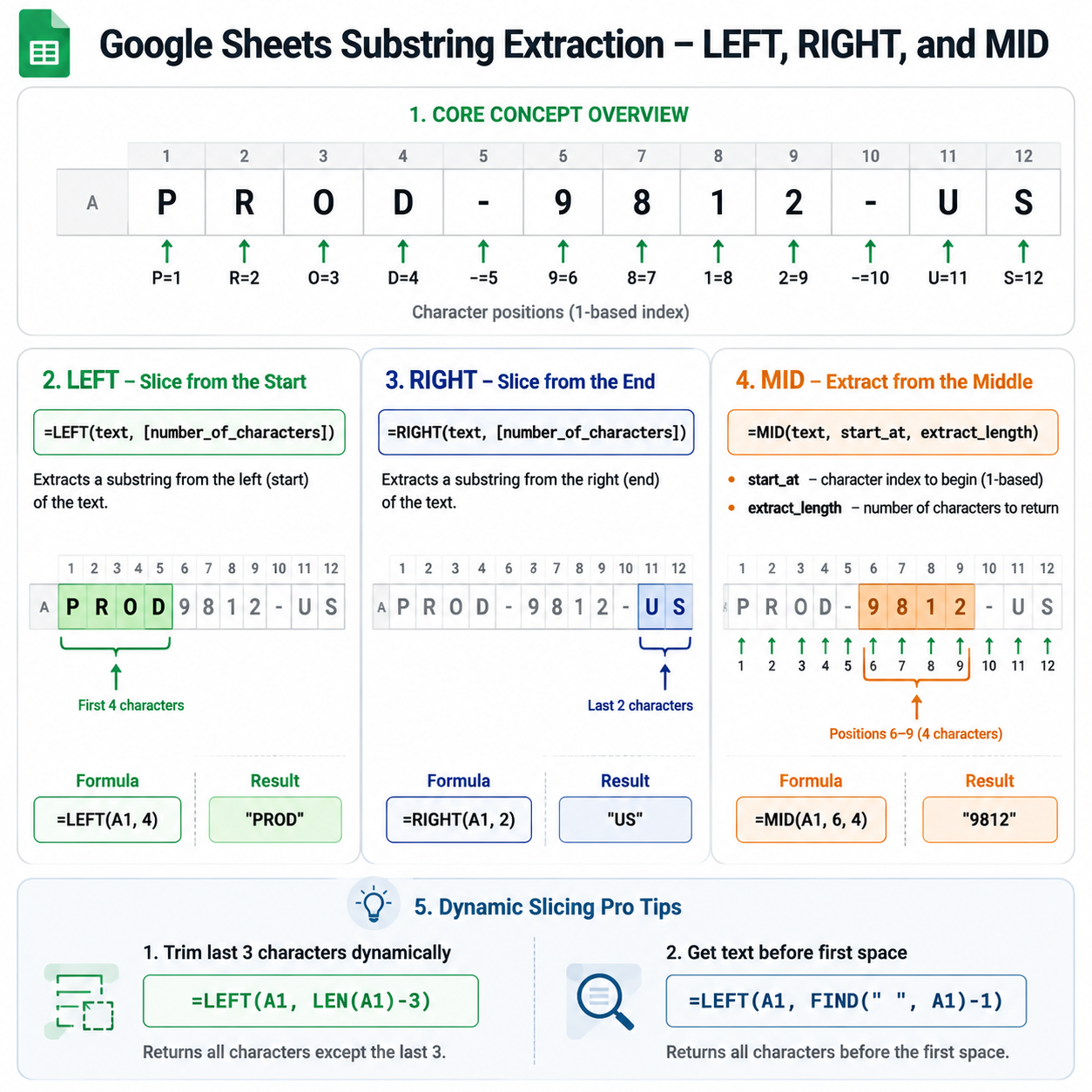
The LEFT function extracts a specified number of characters from the beginning of a text string.
Syntax
=LEFT(text, [number_of_characters])
For example:
=LEFT("Google Sheets", 6)
Result:
Google
The formula takes the first six characters from the text.
Using LEFT with a Cell Reference
Suppose cell A2 contains:
INV-2026-00125
To extract the first three characters:
=LEFT(A2,3)
Result:
INV
This is particularly useful when the beginning of a code represents a category, department, country, or product type.
LEFT Function Examples
| Data | Formula | Result |
|---|---|---|
Google Sheets |
=LEFT(A2,6) |
Google |
INV-2026-00125 |
=LEFT(A2,3) |
INV |
GER-4589 |
=LEFT(A2,3) |
GER |
PROD-1024 |
=LEFT(A2,4) |
PROD |
Quick LEFT Cheat Sheet
=LEFT(A2,3)
Extract the first 3 characters.
=LEFT(A2,5)
Extract the first 5 characters.
=LEFT(A2)
Return the first character because the number of characters defaults to 1.
2. How to Use the RIGHT Function in Google Sheets
The RIGHT function works in the opposite direction.
It extracts a specified number of characters from the end of a text string.
Syntax
=RIGHT(text, [number_of_characters])
For example:
=RIGHT("Google Sheets", 6)
Result:
Sheets
RIGHT Function Example
Suppose A2 contains:
INV-2026-00125
To extract the final five characters:
=RIGHT(A2,5)
Result:
00125
This can be useful when the last part of a code contains a unique identifier.
RIGHT Function Examples
| Data | Formula | Result |
|---|---|---|
Google Sheets |
=RIGHT(A2,6) |
Sheets |
INV-2026-00125 |
=RIGHT(A2,5) |
00125 |
ORDER-98452 |
=RIGHT(A2,5) |
98452 |
PROD-2026-07 |
=RIGHT(A2,2) |
07 |
Quick RIGHT Cheat Sheet
=RIGHT(A2,2)
Extract the last 2 characters.
=RIGHT(A2,4)
Extract the last 4 characters.
=RIGHT(A2,6)
Extract the last 6 characters.
3. How to Use the MID Function in Google Sheets
The MID function is slightly different.
Instead of extracting text from the beginning or end, it allows you to specify:
- Where extraction should start
- How many characters should be extracted
Syntax
=MID(text, starting_at, extract_length)
For example:
=MID("Google Sheets", 8, 6)
Result:
Sheets
The extraction starts at character 8 and continues for 6 characters.
Understanding Character Positions
Let's use:
Google Sheets
The character positions are:
| Position | 1 | 2 | 3 | 4 | 5 | 6 | 7 | 8 | 9 | 10 | 11 | 12 | 13 |
|---|---|---|---|---|---|---|---|---|---|---|---|---|---|
| Character | G | o | o | g | l | e | space | S | h | e | e | t | s |
Therefore:
=MID("Google Sheets",8,6)
starts at position 8 and extracts 6 characters:
Sheets
4. LEFT vs RIGHT vs MID
The easiest way to understand these functions is to compare them directly.
| Function | Direction | Best Used For |
|---|---|---|
| LEFT | From the beginning | Prefixes, codes, country IDs |
| RIGHT | From the end | IDs, suffixes, years, extensions |
| MID | From a specific position | Embedded codes and structured text |
Example
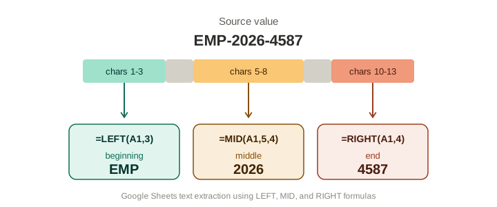
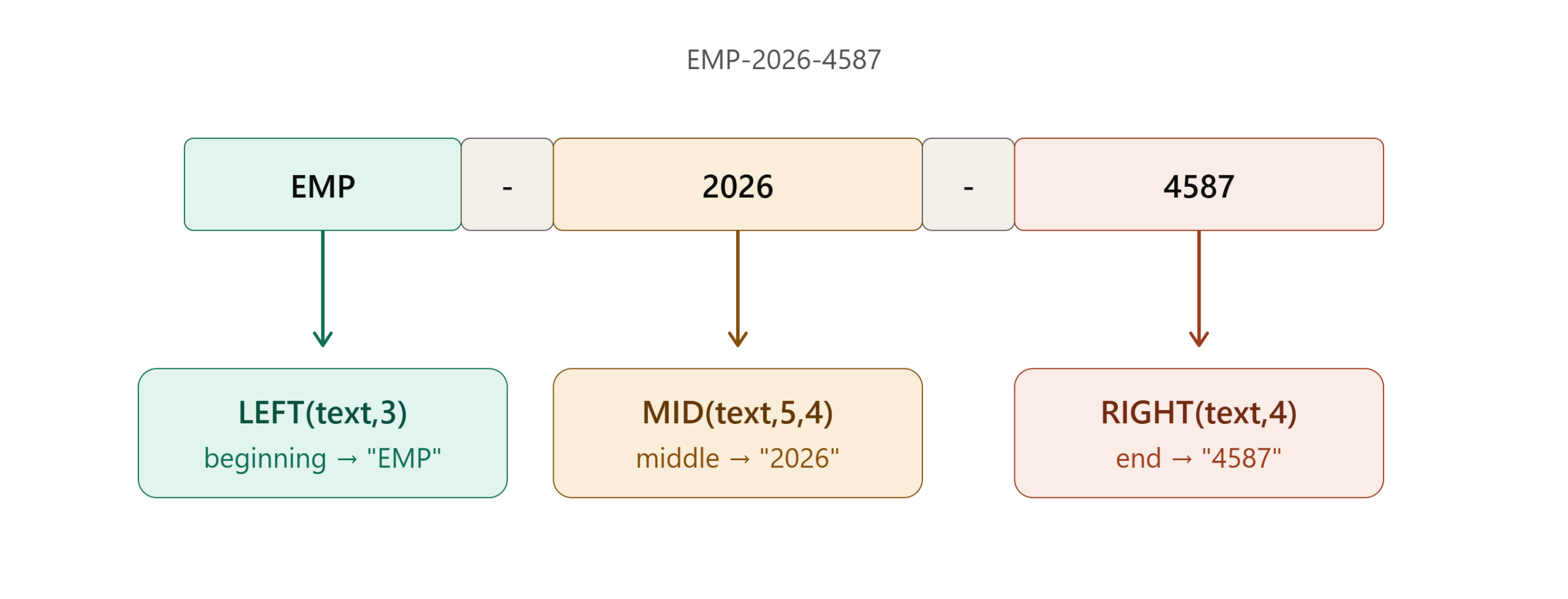
Suppose:
A2 = EMP-2026-4587
You can extract:
Employee prefix:
=LEFT(A2,3)
Result:
EMP
Year:
=MID(A2,5,4)
Result:
2026
Employee number:
=RIGHT(A2,4)
Result:
4587
One cell has been transformed into three useful pieces of information.
5. Real-World Google Sheets Examples
These functions are especially useful for business spreadsheets.
Example 1: Extract a Country Code
Suppose your customer IDs look like:
GER-45892
FRA-38472
USA-72931
Use:
=LEFT(A2,3)
You can then create a separate Country Code column.
Example 2: Extract a Product ID
Suppose product codes are:
PRODUCT-45892
PRODUCT-72913
PRODUCT-84125
Use:
=RIGHT(A2,5)
Result:
45892
72913
84125
Example 3: Extract the Year from an Order Code
Suppose your order numbers are:
ORD-2026-00125
ORD-2025-00892
ORD-2024-01542
The year begins at character 5.
Use:
=MID(A2,5,4)
Result:
2026
2025
2024
6. Extract Information from Email Addresses
LEFT, RIGHT, and MID can also help process email addresses.
Suppose:
A2 = john.smith@example.com
To extract everything before the @ symbol, however, using a delimiter-based function such as LEFT with FIND is more flexible than hard-coding the number of characters.
Use:
=LEFT(A2,FIND("@",A2)-1)
Result:
john.smith
To extract the domain:
=RIGHT(A2,LEN(A2)-FIND("@",A2))
Result:
example.com
This demonstrates an important concept:
LEFT and RIGHT become much more powerful when combined with other Google Sheets functions.
7. Combine LEFT, RIGHT, and MID with Other Functions
The real power of these functions appears when you combine them with functions such as:
FINDSEARCHLENTRIMSUBSTITUTEIFARRAYFORMULA
LEFT + FIND
Extract everything before a hyphen:
=LEFT(A2,FIND("-",A2)-1)
If A2 contains:
Marketing-2026
The result is:
Marketing
RIGHT + FIND
Extract everything after a hyphen:
=RIGHT(A2,LEN(A2)-FIND("-",A2))
Result:
2026
MID + FIND
MID can be used when the desired text is located between two delimiters.
For example:
EMP-2026-4587
To extract the year:
=MID(A2,FIND("-",A2)+1,4)
Result:
2026
8. LEFT, RIGHT, and MID for Data Cleaning
Data cleaning is one of the most common spreadsheet tasks where these functions become useful.
Imagine importing a dataset containing:
Customer ID
GER-00125
GER-00126
USA-00231
FRA-00842
You can create separate columns:
| Customer ID | Country | Customer Number |
|---|---|---|
| GER-00125 | GER | 00125 |
| USA-00231 | USA | 00231 |
| FRA-00842 | FRA | 00842 |
Country:
=LEFT(A2,3)
Customer number:
=RIGHT(A2,5)
This makes the original dataset much easier to filter, sort, analyze, and visualize.
9. Use ARRAYFORMULA to Process an Entire Column
If you have hundreds or thousands of rows, manually copying formulas isn't efficient.
For example:
=ARRAYFORMULA(IF(A2:A="","",LEFT(A2:A,3)))
This can apply the LEFT operation across the column.
Similarly:
=ARRAYFORMULA(IF(A2:A="","",RIGHT(A2:A,5)))
And:
=ARRAYFORMULA(IF(A2:A="","",MID(A2:A,5,4)))
This is particularly useful for automated Google Sheets workflows.
10. Common LEFT, RIGHT, and MID Mistakes
Mistake 1: Counting Characters Incorrectly
Suppose:
ABC-2026
You might assume that the year starts at position 4.
It doesn't.
The hyphen occupies position 4.
The year starts at position 5.
Use:
=MID(A2,5,4)
Mistake 2: Forgetting Spaces
Consider:
John Smith
There is a space between the first and last name.
Spaces count as characters.
Therefore:
=LEFT(A2,4)
returns:
John
but:
=MID(A2,6,5)
returns:
Smith
Mistake 3: Using a Fixed Number When the Data Changes
This formula:
=LEFT(A2,5)
works only when the information you want always occupies the first five characters.
If the text structure changes, use delimiter-based functions such as FIND or SEARCH.
For example:
=LEFT(A2,FIND("-",A2)-1)
is more flexible for extracting everything before the first hyphen.
11. LEFT, RIGHT, and MID Cheat Sheet
Here's the quick-reference section you can bookmark.
| Task | Formula |
|---|---|
| First 3 characters | =LEFT(A2,3) |
| First 5 characters | =LEFT(A2,5) |
| Last 3 characters | =RIGHT(A2,3) |
| Last 5 characters | =RIGHT(A2,5) |
| Characters 5–8 | =MID(A2,5,4) |
Text before - |
=LEFT(A2,FIND("-",A2)-1) |
Text after - |
=RIGHT(A2,LEN(A2)-FIND("-",A2)) |
Text before @ |
=LEFT(A2,FIND("@",A2)-1) |
Text after @ |
=RIGHT(A2,LEN(A2)-FIND("@",A2)) |
| LEFT across a column | =ARRAYFORMULA(IF(A2:A="","",LEFT(A2:A,3))) |
| RIGHT across a column | =ARRAYFORMULA(IF(A2:A="","",RIGHT(A2:A,5))) |
12. A Simple Way to Remember the Three Functions
If you're learning Google Sheets formulas, remember this:
LEFT
Start → move right
LEFT(A2, number)
RIGHT
End → move left
RIGHT(A2, number)
MID
Choose a position → extract a number of characters
MID(A2, start, number)
Once this mental model becomes familiar, you'll be able to choose the correct function almost immediately.
13. When Should You Use LEFT, RIGHT, or MID?
Use LEFT when the information you need is at the beginning.
Examples:
- Country codes
- Department codes
- Product prefixes
- Employee prefixes
Use RIGHT when the information is at the end.
Examples:
- Order numbers
- Product IDs
- File extensions
- Year or month codes
Use MID when the information is embedded inside the text.
Examples:
- Years inside order codes
- Category codes
- Account numbers
- Structured IDs
If the position of the information changes between rows, combine these functions with FIND, SEARCH, or other text functions.
Conclusion
The LEFT, RIGHT, and MID functions in Google Sheets are simple, but they can save a significant amount of time when working with structured text.
You can use them to:
- Extract IDs
- Clean imported data
- Separate codes
- Process customer information
- Analyze product numbers
- Standardize datasets
- Prepare data for dashboards
- Automate repetitive spreadsheet tasks
The key is to understand the difference:
LEFT = beginning
RIGHT = end
MID = specific position
Once you've mastered these three functions, combine them with FIND, LEN, SEARCH, IF, and ARRAYFORMULA to build more flexible spreadsheet workflows.
If you work with Google Sheets regularly, save this page as a reference and explore our other Google Sheets formulas, automation, and Google Workspace productivity guides to take your spreadsheets further.
Frequently Asked Questions
What is the LEFT function in Google Sheets?
The LEFT function extracts a specified number of characters from the beginning of a text string.
Example:
=LEFT(A2,3)
returns the first three characters from A2.
What is the RIGHT function in Google Sheets?
The RIGHT function extracts a specified number of characters from the end of a text string.
Example:
=RIGHT(A2,5)
returns the last five characters from A2.
What is the MID function in Google Sheets?
The MID function extracts characters from a specific position within a text string.
Example:
=MID(A2,5,4)
starts at character 5 and extracts four characters.
What is the difference between LEFT, RIGHT, and MID?
LEFT extracts characters from the beginning, RIGHT extracts characters from the end, and MID extracts characters from a specified position.
Can LEFT, RIGHT, and MID be used with ARRAYFORMULA?
Yes. These functions can be combined with ARRAYFORMULA to process multiple rows automatically.
For example:
=ARRAYFORMULA(IF(A2:A="","",LEFT(A2:A,3)))
How can I extract text before a character in Google Sheets?
You can combine LEFT with FIND.
For example:
=LEFT(A2,FIND("-",A2)-1)
This extracts everything before the first hyphen.
How can I extract text after a character in Google Sheets?
You can combine RIGHT, LEN, and FIND.
For example:
=RIGHT(A2,LEN(A2)-FIND("-",A2))
This extracts everything after the first hyphen.
Related Google Sheets Resources
You may also be interested in:
- VLOOKUP Cheat Sheet
- XLOOKUP Cheat Sheet
- QUERY Function Cheat Sheet
- FILTER Function Cheat Sheet
- ARRAYFORMULA Cheat Sheet
- IF Function Cheat Sheet
- SUM Cheat Sheet
- SUMIF Cheat Sheet
- COUNTIF Cheat Sheet
- IMPORTRANGE Cheat Sheet