

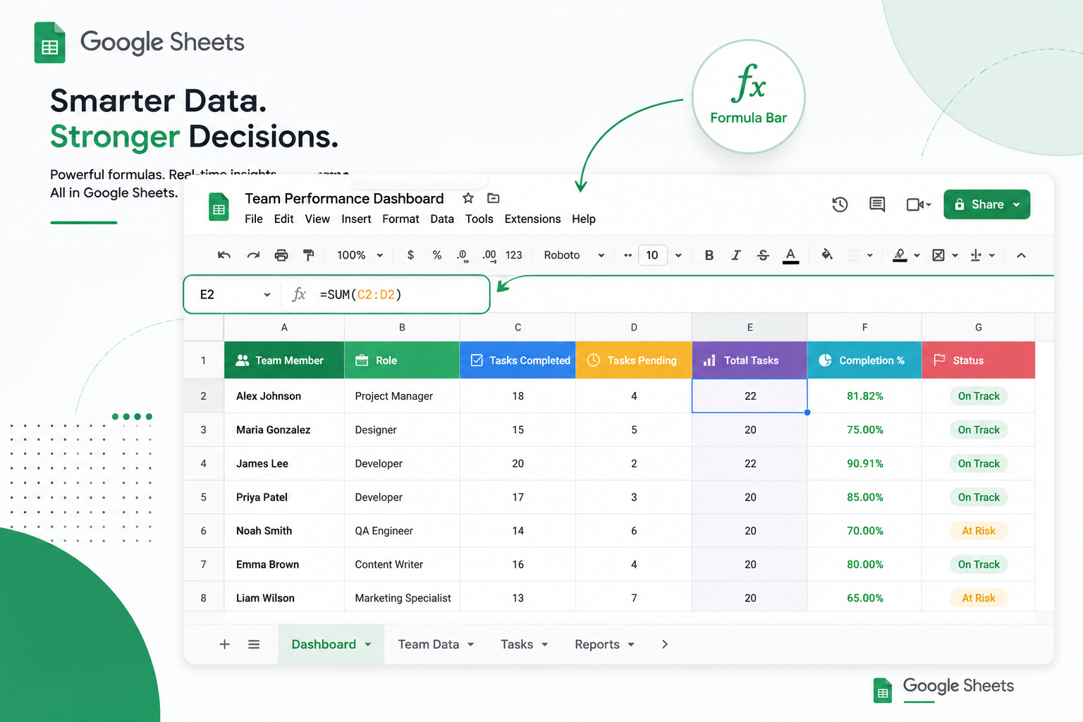
7 Google Sheets Formulas That Replace Entire Excel Add-Ons

7 Google Sheets Formulas That Replace Entire Excel Add-Ons
Google Sheets tab bar
If you migrated to Google Workspace from Excel, you probably brought a habit with you: reaching for a paid add-on every time you needed something more than SUM and VLOOKUP. Pivot table add-ins, web-scraping plugins, currency converters, text-parsing tools — the Excel add-on marketplace exists because native Excel formulas only get you so far.
Google Sheets is different. A handful of its built-in functions were designed to do the job of entire add-on categories, with no installation, no per-seat licensing, and no security review from your IT team. For teams already living inside Google Workspace collaboration tools, that matters: fewer third-party scripts touching your data, fewer approvals to chase, and one less line item in the software budget.
This post walks through seven formulas that consistently replace add-ons professionals swear by in Excel. Each one includes the syntax, a real business scenario, and where relevant, a step-by-step walkthrough you can follow along with in your own sheet.
Quick Reference: What Each Formula Replaces
| Formula | Excel Add-On It Replaces | Best For |
|---|---|---|
QUERY |
Pivot table / SQL add-ins | Filtering, grouping, and summarizing large datasets |
IMPORTRANGE |
Data consolidation tools (e.g., Power Query cross-file merges) | Pulling live data from other spreadsheets |
GOOGLEFINANCE |
Stock/market data plugins | Live stock prices, currency conversion, historical data |
REGEXEXTRACT / REGEXREPLACE |
Text-parsing add-ins | Cleaning messy exports, extracting patterns from text |
SPARKLINE |
Mini-chart / in-cell visualization add-ons | Compact trend visuals inside a single cell |
IMPORTXML / IMPORTHTML |
Web-scraping add-ins | Pulling structured data from public web pages |
ARRAYFORMULA |
Bulk-calculation / “fill down” automation add-ins | Applying one formula across an entire column instantly |
1. QUERY — Your Built-In Pivot Table and SQL Engine
Replaces: Pivot table add-ins, SQL-style reporting plugins
QUERY lets you filter, sort, group, and aggregate data using a syntax borrowed from SQL. Instead of building a pivot table and refreshing it manually, you write one formula that updates live as your source data changes.
Syntax:
=QUERY(data, query, [headers])
Business scenario: A sales team tracks deals in a raw export from their CRM — hundreds of rows, no summary view. Instead of rebuilding a pivot table every Monday, the sales ops lead writes:
=QUERY(Deals!A1:F1000, "SELECT C, SUM(E) WHERE D = 'Closed Won' GROUP BY C ORDER BY SUM(E) DESC", 1)
This instantly returns total closed-won revenue by sales rep, sorted highest to lowest, and it updates automatically every time the CRM export refreshes the source tab.
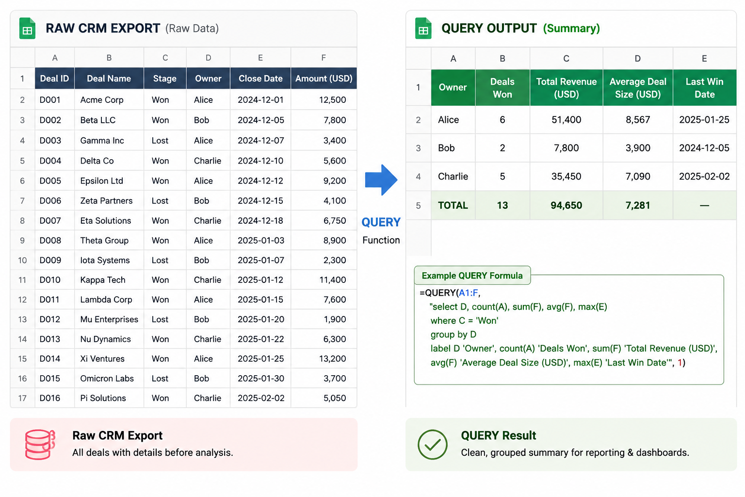
QUERY Function
Step-by-Step: Building Your First QUERY Report
- Organize your source data into a single tab with clear column headers in row 1 — QUERY needs consistent columns to reference correctly.
- Pick an empty cell on a new tab where you want the summary to appear (keeping reports separate from raw data prevents accidental overwrites).
- Start the formula with
=QUERY(and select your full data range, including headers, e.g.Deals!A1:F1000. - Write your query string in quotes using SQL-style clauses:
SELECT,WHERE,GROUP BY,ORDER BY. - Set the headers argument — usually
1if your data has one header row. - Press Enter. Adjust the
SELECTcolumns orWHEREconditions until the output matches what you need. - Reference this summary tab in dashboards or charts, so those visuals update automatically whenever new deals are added.
Query Function Cheat Sheet [Click Here]
2. IMPORTRANGE — Live Cross-Spreadsheet Consolidation
Replaces: Data consolidation and cross-workbook merge add-ins
In Excel, pulling live data from another workbook usually means an add-on or a fragile external reference. IMPORTRANGE does this natively, pulling a live, auto-updating range from any other Google Sheet you have access to.
Syntax:
=IMPORTRANGE("spreadsheet_url", "range_string")
Business scenario: Each regional manager keeps their own expense tracker. Finance needs one consolidated view without asking anyone to copy-paste data weekly. A single master sheet uses:
=IMPORTRANGE("https://docs.google.com/spreadsheets/d/EAST_REGION_ID", "Expenses!A2:F")
repeated for each region, and finance always sees current numbers — no manual consolidation, no version confusion over “which file is the latest.”
Note for IT admins: The first time
IMPORTRANGEconnects two sheets, it requires explicit permission approval. This is a feature, not a bug — it means cross-sheet data access is auditable and consent-based, which matters if you’re managing this through the Google Workspace admin console.
IMPORTRANGE Function Cheat Sheet [Click Here]
3. GOOGLEFINANCE — Real-Time Market Data, No Plugin Required
Replaces: Stock ticker and currency-conversion add-ins
GOOGLEFINANCE pulls current and historical stock prices, exchange rates, and market data directly into a cell.
Syntax:
=GOOGLEFINANCE(ticker, [attribute], [start_date], [end_date|num_days], [interval])
Business scenario: An operations team pays international contractors and needs to budget in USD despite invoices arriving in EUR. Instead of manually checking exchange rates:
=B2 * GOOGLEFINANCE("CURRENCY:EURUSD")
converts the invoice amount automatically, and the conversion rate updates every time the sheet is opened — no separate currency add-on, no stale rates.
4. REGEXEXTRACT and REGEXREPLACE — Text Cleanup Without a Plugin
Replaces: Text-parsing and data-cleaning add-ins
Messy exports are the norm — inconsistent formatting, extra characters, values buried inside longer strings. REGEXEXTRACT pulls out exactly the pattern you need; REGEXREPLACE finds and replaces based on a pattern rather than an exact match.
Syntax:
=REGEXEXTRACT(text, regular_expression)
=REGEXREPLACE(text, regular_expression, replacement)
Business scenario: A support team exports tickets where the customer’s order number is buried inside a subject line like "Re: Order #48213 - Shipping delay". Rather than manually copying order numbers into a new column:
=REGEXEXTRACT(A2, "#(\d+)")
extracts just 48213 from every row at once — a task that would otherwise require a dedicated text-parsing add-on or a manual find-and-replace pass.
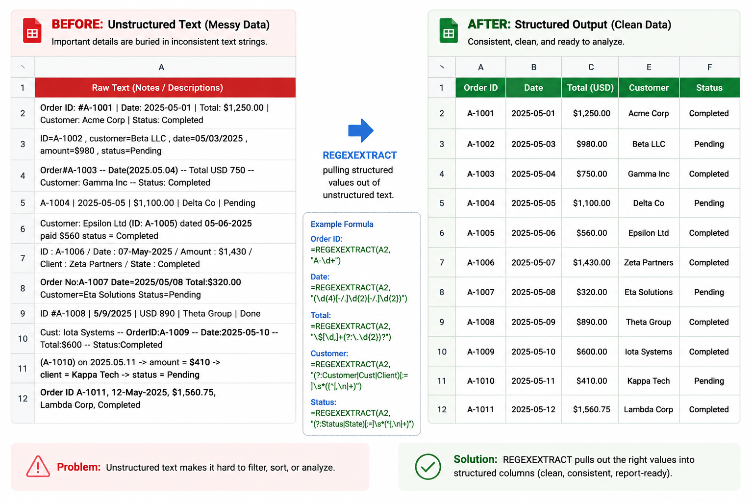
REGEXEXTRACT
5. SPARKLINE — In-Cell Charts Without a Visualization Add-On
Replaces: Mini-chart and in-cell visualization plugins
SPARKLINE draws a small chart — line, bar, column, or win/loss — directly inside a single cell. It’s the fastest way to show a trend inside a dashboard or report without building a full chart object.
Syntax:
=SPARKLINE(data, [options])
Business scenario: A team lead builds a weekly status dashboard and wants to show each project’s progress trend at a glance, next to its name, without cluttering the sheet with a dozen separate charts:
=SPARKLINE(B2:M2, {"charttype","column";"color","#B9F53C"})
renders a compact column chart of 12 weeks of progress data, right inside the cell next to the project name.
6. IMPORTXML and IMPORTHTML — Native Web Scraping
Replaces: Web-scraping and data-extraction add-ins
Need to pull a table from a public webpage, or a specific value from a page’s structure? IMPORTHTML grabs tables or lists; IMPORTXML grabs specific elements using XPath.
Syntax:
=IMPORTHTML(url, "table"|"list", index)
=IMPORTXML(url, xpath_query)
Business scenario: A market research analyst tracks competitor pricing published on a public pricing page. Instead of manually checking the page weekly:
=IMPORTXML("https://example.com/pricing", "//span[@class='price']")
pulls the current listed price directly into the sheet, refreshing automatically — the same job a paid scraping add-on would otherwise handle.
Use responsibly: Only import from pages you have the right to access and pull from — respect a site’s terms of service and
robots.txt, and avoid scraping data behind login walls or paywalls.
7. ARRAYFORMULA — Apply One Formula to an Entire Column, Instantly
Replaces: Bulk-calculation and “auto-fill down” automation add-ins
Normally, applying a formula to a whole column means writing it once and dragging it down — and remembering to redo that every time a new row is added. ARRAYFORMULA applies a single formula across an entire range at once, and automatically extends to new rows.
Syntax:
=ARRAYFORMULA(expression)
Business scenario: A finance team calculates commission on every row of a growing sales log. Instead of dragging a formula down every time new rows are added:
=ARRAYFORMULA(IF(B2:B="", "", B2:B * 0.1))
calculates commission for every existing row and automatically applies to new rows as they’re added — turning a recurring manual task into a one-time setup.
ARRAYFORMULA Cheat Sheet [Click Here]
Putting It Together: A CRM Dashboard Example
Here’s how several of these formulas stack in a real internal tool: a lightweight CRM dashboard built in Google Sheets instead of a paid CRM platform.
QUERYbuilds the summary tables (deals by stage, revenue by rep).IMPORTRANGEpulls in data logged by different team members across separate sheets.SPARKLINEshows each rep’s weekly deal trend inline.ARRAYFORMULAcalculates commission and deal-aging columns automatically as new rows come in.REGEXEXTRACTcleans up lead source data pulled from a marketing export.
That’s five paid-add-on categories replaced by native formulas in a single internal tool — with the added benefit that everything lives inside your team’s existing Google Workspace collaboration tools, with sharing and permissions already handled.
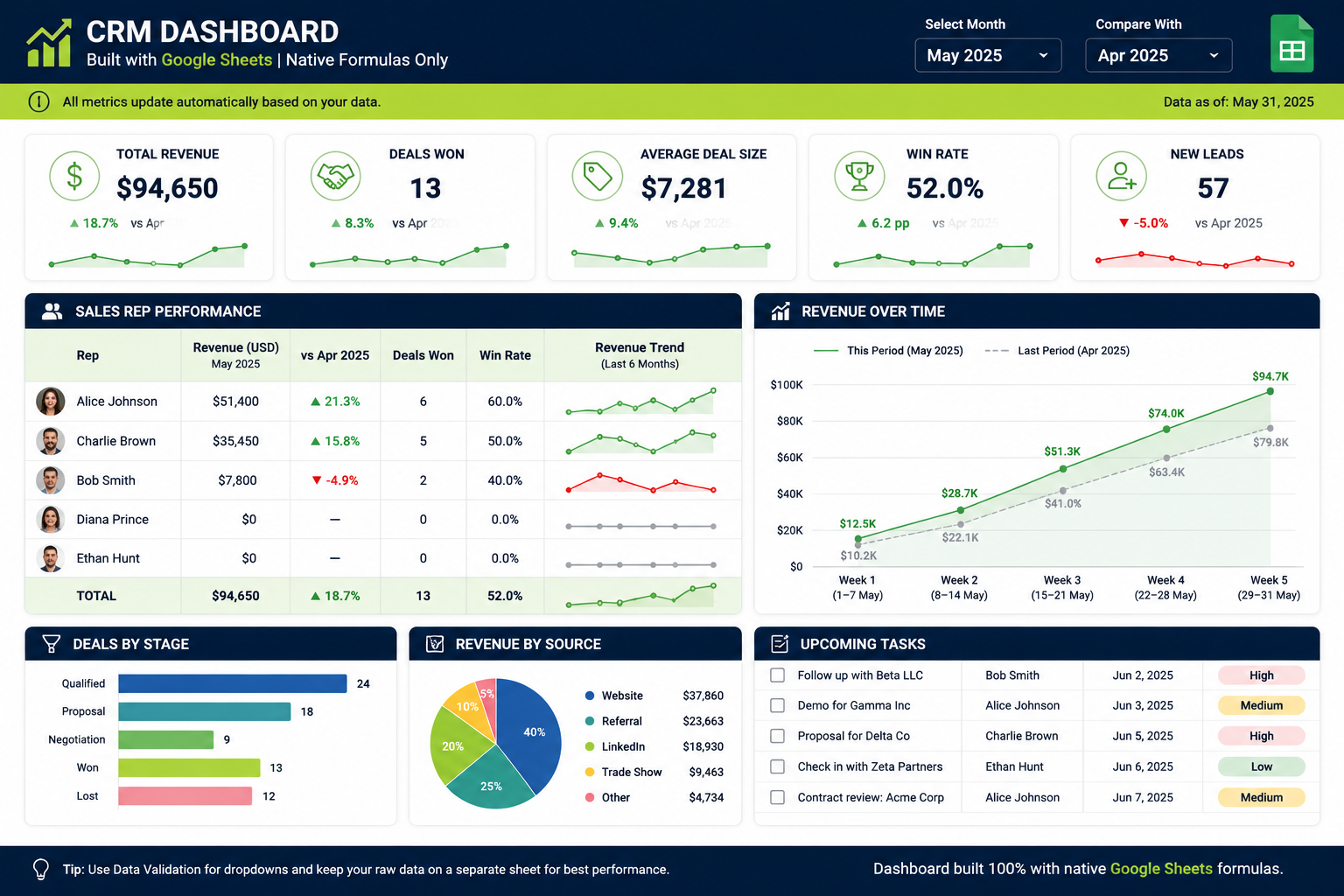
CRM Dashboard
Key Takeaways
- QUERY replaces pivot tables and SQL-style reporting add-ins with one live formula.
- IMPORTRANGE consolidates data across spreadsheets without manual copy-paste.
- GOOGLEFINANCE delivers live market and currency data with zero setup.
- REGEXEXTRACT / REGEXREPLACE clean and parse messy text natively.
- SPARKLINE adds in-cell trend visuals without a charting add-on.
- IMPORTXML / IMPORTHTML pull structured web data directly into your sheet.
- ARRAYFORMULA eliminates manual drag-to-fill work, permanently.
None of these require IT approval, a subscription, or a plugin review — which makes them a natural starting point if your organization is trying to standardize on native Google Workspace collaboration tools and reduce the number of third-party scripts with access to company data.
Try it this week: Pick one recurring report you currently rebuild manually — a weekly summary, a status dashboard, a data cleanup pass — and rebuild it using one formula from this list. Most teams find their first QUERY report alone pays for the time investment within a month.
Keep Reading
- Google Sheets Advanced Functions: Unlocking the Power of Spreadsheets
- How to Limit Responses in Google Forms: The Complete Guide (2026 Update)
- The Ultimate Guide to High-Conversion Google Forms: From Data Collection to Behavioral Science
Call to Action
Ready to level up your Google Workspace productivity?
For more productivity tips, explore our related guides:
YouTube Channel: https://www.youtube.com/@TechTrickswithEli2023
Telegram Channel: https://t.me/techtrickswithEli